PINNs in Practice: From First Principles to PyTorch
TL;DR. Physics-Informed Neural Networks (PINNs) solve differential equations by turning the PDE residual and boundary/initial conditions into a loss that a neural network minimizes via automatic differentiation. Below is a minimal but rigorous primer—with proofs, pictures, and runnable PyTorch.
1) What is a PINN?
Given a PDE
\[ \mathcal{N}[u](\mathbf{x}) = f(\mathbf{x}) \ \text{in }\Omega,\qquad \mathcal{B}[u](\mathbf{x}) = g(\mathbf{x}) \ \text{on }\partial\Omega, \]
a PINN represents \(u_\theta(\mathbf{x})\) with a neural net and trains \(\theta\) to minimize a physics-driven objective:
\[ \mathcal{L}(\theta)= \lambda_{\mathrm{pde}}\frac{1}{N_\Omega}\sum_{i=1}^{N_\Omega}\big\|\mathcal{N}[u_\theta](\mathbf{x}_i)-f(\mathbf{x}_i)\big\|^2+ \lambda_{\mathrm{bc}}\frac{1}{N_{\partial\Omega}}\sum_{j=1}^{N_{\partial\Omega}}\big\|\mathcal{B}[u_\theta](\mathbf{x}_j)-g(\mathbf{x}_j)\big\|^2. \]
All derivatives in \(\mathcal{N}\) and \(\mathcal{B}\) are obtained by automatic differentiation through the network. For background and canonical formulations, see Raissi–Perdikaris–Karniadakis and the Nat Rev Phys overview of physics-informed ML [1, 2].
2) A tiny existence/uniqueness checkpoint (Poisson, Dirichlet)
Consider Poisson’s equation with Dirichlet BCs:
\[ -\Delta u = f \ \text{in }\Omega,\qquad u = 0 \ \text{on }\partial\Omega. \]
Weak form: find \(u\in H^1_0(\Omega)\) with \(a(u,v)=\ell(v)\) for all \(v\in H^1_0(\Omega)\), where \(a(u,v)=\int_\Omega \nabla u\cdot\nabla v \, dx\), \(\ell(v)=\int_\Omega f v \, dx\). By Poincaré inequality, \(a\) is coercive/continuous, so Lax–Milgram gives existence/uniqueness; choosing \(v=u\) yields \(\|\nabla u\|_2^2 = \ell(u)\) and the standard energy uniqueness. This underpins why driving the strong residual and BC mismatch to zero is a consistent surrogate for the weak solution in PINNs (assuming expressive nets and adequate sampling). See [2].
3) Pictures to anchor intuition
- Burgers’ equation (shock formation; a staple PINN benchmark). Background & formulas here [5].

- Method of images (intuition for Laplace/Poisson boundary effects) [7].
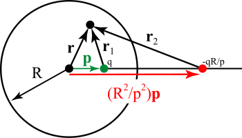
Images are from Wikipedia; keep attribution if you reuse outside the blog.
4) Minimal PyTorch PINN: 1D Poisson \(-u''=\pi^2\sin(\pi x)\), \(u(0)=u(1)=0\)
True solution: \(u^\star(x)=\sin(\pi x)\).
import torch, math
from torch import nn

device = "cuda" if torch.cuda.is_available() else "cpu"
torch.manual_seed(0)

# ----- network -----
class MLP(nn.Module):
    def __init__(self, in_dim=1, out_dim=1, width=64, depth=4):
        super().__init__()
        layers = [nn.Linear(in_dim, width), nn.Tanh()]
        for _ in range(depth-1):
            layers += [nn.Linear(width, width), nn.Tanh()]
        layers += [nn.Linear(width, out_dim)]
        self.net = nn.Sequential(*layers)
    def forward(self, x):
        return self.net(x)

net = MLP().to(device)

# ----- collocation sampling -----
def sample_interior(n):
    x = torch.rand(n, 1, device=device)  # (0,1)
    x.requires_grad_(True)
    return x

def sample_boundary(n_each=128):
    xb0 = torch.zeros(n_each, 1, device=device, requires_grad=True)
    xb1 = torch.ones(n_each, 1, device=device, requires_grad=True)
    return xb0, xb1

# RHS f(x) = pi^2 sin(pi x)
def f(x): return (math.pi**2) * torch.sin(math.pi * x)

# ----- residuals via autograd -----
def pde_residual(x):
    u = net(x)
    du = torch.autograd.grad(u, x, grad_outputs=torch.ones_like(u),
                             create_graph=True)[0]
    d2u = torch.autograd.grad(du, x, grad_outputs=torch.ones_like(du),
                              create_graph=True)[0]
    # -u'' = f  => residual r = -u'' - f
    r = -d2u - f(x)
    return r

# ----- loss -----
def loss_fn(n_int=1024, n_b=128, w_pde=1.0, w_bc=10.0):
    xi = sample_interior(n_int)
    xb0, xb1 = sample_boundary(n_b)
    r = pde_residual(xi)
    u0 = net(xb0); u1 = net(xb1)
    return (w_pde * (r**2).mean()
            + w_bc * (u0**2).mean()
            + w_bc * (u1**2).mean())

opt = torch.optim.Adam(net.parameters(), lr=1e-3)

# ----- train -----
for step in range(4000):
    opt.zero_grad()
    L = loss_fn()
    L.backward()
    opt.step()
    if step % 500 == 0:
        print(f"step {step:4d}  loss {L.item():.3e}")

# quick check (L2 error on grid)
with torch.no_grad():
    xg = torch.linspace(0,1,401, device=device).unsqueeze(1)
    err = torch.sqrt(((net(xg) - torch.sin(math.pi*xg))**2).mean())
    print("L2 grid error ~", err.item())
For a MATLAB reference implementation of Poisson PINNs (nice for sanity checks), see the official example [7].
5) Time-dependent PINN: 1D viscous Burgers \(u_t + u u_x - \nu u_{xx}=0\)
import torch, math
from torch import nn

device = "cuda" if torch.cuda.is_available() else "cpu"
torch.manual_seed(42)

# domain: x in [-1,1], t in [0,1], IC u(x,0)= -sin(pi x), BC u(-1,t)=u(1,t)=0
nu = 0.01 / math.pi

class MLP2D(nn.Module):
    def __init__(self, width=128, depth=6):
        super().__init__()
        layers = [nn.Linear(2, width), nn.Tanh()]
        for _ in range(depth-1):
            layers += [nn.Linear(width, width), nn.Tanh()]
        layers += [nn.Linear(width, 1)]
        self.net = nn.Sequential(*layers)
    def forward(self, xt):
        return self.net(xt)

net = MLP2D().to(device)

def sample_rect(n):
    x = -1 + 2*torch.rand(n, 1, device=device)
    t = torch.rand(n, 1, device=device)
    xt = torch.cat([x, t], dim=1).requires_grad_(True)
    return xt

def sample_ic(n):
    x = -1 + 2*torch.rand(n, 1, device=device)
    t = torch.zeros_like(x)
    xt = torch.cat([x, t], dim=1).requires_grad_(True)
    u0 = -torch.sin(math.pi*x)
    return xt, u0

def sample_bc(n):
    t = torch.rand(n, 1, device=device)
    xm = -torch.ones_like(t); xp = torch.ones_like(t)
    xtm = torch.cat([xm, t], dim=1).requires_grad_(True)
    xtp = torch.cat([xp, t], dim=1).requires_grad_(True)
    return xtm, xtp

def burgers_residual(xt):
    xt.requires_grad_(True)
    u = net(xt)
    du = torch.autograd.grad(u, xt, torch.ones_like(u), create_graph=True)[0]
    u_x = du[:, :1]; u_t = du[:, 1:]
    u_xx = torch.autograd.grad(u_x, xt, torch.ones_like(u_x), create_graph=True)[0][:, :1]
    r = u_t + u * u_x - nu * u_xx
    return r

opt = torch.optim.Adam(net.parameters(), lr=1e-3)

def loss():
    r = burgers_residual(sample_rect(2048))
    xt_ic, u0 = sample_ic(512)
    u_ic = net(xt_ic)
    xtm, xtp = sample_bc(256)
    u_m = net(xtm); u_p = net(xtp)
    return (r.pow(2).mean()
            + 10.0 * (u_ic - u0).pow(2).mean()
            + 10.0 * (u_m**2).mean()
            + 10.0 * (u_p**2).mean())

for step in range(5000):
    opt.zero_grad()
    L = loss()
    L.backward()
    opt.step()
    if step % 500 == 0:
        print(step, L.item())
A concise background on Burgers (inviscid/viscous forms, Cole–Hopf) is here [5].
6) Where PINNs sit vs neural operators (context)
PINNs hard-enforce physics via residuals/BC losses; neural operators (e.g., FNO, DeepONet) learn solution operators from data and can be extremely fast once trained. See FNO and DeepONet for complementary approaches and trade-offs [3,4].
7) Practical tips
- Sampling: Mix uniform + boundary-biased + residual-adaptive points; curriculum in time for transients.
- Loss balancing: Start with larger BC/IC weight; consider gradient-norm balancing.
- Architectures: Tanh/SIREN for smooth/oscillatory fields; Fourier features for multiscale.
- Stiffness: For shocks, upweight diffusion, oversample near gradients, or hybridize with classical data.
- Validation: Always compare to a reference solver mesh and report \(L^2\)/\(H^1\) errors.
For broader reviews and recent advances, see the 2021 Nature Reviews Physics survey and newer reviews in fluids/applied sciences [2,8,9].
References (Harvard style)
- Raissi, M., Perdikaris, P. and Karniadakis, G.E., 2019. Physics-informed neural networks: A deep learning framework for solving forward and inverse problems involving nonlinear partial differential equations. Journal of Computational Physics, 378, pp.686–707. Available at: link.
- Karniadakis, G.E., Kevrekidis, I.G., Lu, L., Perdikaris, P., Wang, S. and Yang, L., 2021. Physics-informed machine learning. Nature Reviews Physics, 3(6), pp.422–440. Available at: link.
- Li, Z., Kovachki, N., Azizzadenesheli, K., Liu, B., Bhattacharya, K., Stuart, A. and Anandkumar, A., 2021. Fourier Neural Operator for Parametric Partial Differential Equations. ICLR 2021. Available at: arXiv.
- Lu, L., Jin, P. and Karniadakis, G.E., 2021. Learning nonlinear operators via DeepONet based on the universal approximation theorem of operators. Nature Machine Intelligence, 3(3), pp.218–229. Available at: PDF.
- Burgers’ equation. 2024. Wikipedia. Available at: link. (Accessed 16 Oct 2025).
- Method of images. 2024. Wikipedia. Available at: link. (Accessed 16 Oct 2025).
- MathWorks, 2023. Solve Poisson Equation on Unit Disk Using Physics-Informed Neural Networks (PINN). Available at: link. (Accessed 16 Oct 2025).
- Xu, H., Zhang, Y., Lin, W., Liu, Y. and Wang, Q., 2024. A comprehensive review of advances in physics-informed neural networks for fluid dynamics. Physics of Fluids, 36(10), 101301. Available at: link.
- Wang, Y., Chen, X. and Zhou, Y., 2025. Physics-Informed Neural Networks: A Review of Methodological Evolution and Frontiers. Applied Sciences, 15(14), 8092. Available at: link.